Elections of 2018: Factor X and "saw Churov"

The presidential election on March 18, 2018 was held with the official explicit of voters (the share of voters who received ballots from all registered voters) 67.54%. The result of the winner - V. Putin - amounted to 76.69%; Officially, 51.77% of the total number of registered voters voted for him. But what is the analysis of electoral statistics tell us about?

The current elected campaign was largely unique. Against the backdrop of the preceding Duma elections of 2016, marked by an unprecedentedly low explicit and an extremely strange distribution of votes (see [1]), unprecedented efforts were made to attract voters to sections - from massive campaigning in the elections to the introduction of a new voting system at the place of residence. This innovation, on the one hand, facilitated such a vote for voters, and on the other, apparently, it facilitated administrative control over voting by employers (primarily budgetary organizations) and other parties interested in the high expense of the parties.

These efforts had borne - the official turnout exceeded the indicators of 2004 and 2012, the result of the winner exceeded the 2004 record, and the absolute number of the 2008 previous record of the winner.

The author published by the author previously analyzed the detailed data of the past federal elections in Russia [2] showed that polling stations with abnormal voting indicators make a significant contribution to the turnout and the result of the winner to suspect the presence of falsifications.

In recent years, thanks to the widespread development of the observation movement and the emergence of video surveillance in polling stations, many evidence has appeared that these suspicions have a material basis. For example, a large-scale study of video recordings of the 2016 State Duma at the polling stations of Kazan, conducted by the Association of Tatarstan observers, showed that the real appearance in the city sections is ten percentage points below the official and close to the turnout in other large cities, including Moscow and St. Petersburg [3].

A similar analysis of voting video recordings in the 2012 presidential elections in the Tatarstan district center Nurlat showed that, contrary to official data (according to which the provincial Tatarstan traditionally votes with the appearance and result of the chief candidate, close to 100%), the actual appearance of voters in the polls of this city was close to Moscow or St. Petersburg [4].

Used data

At the time of preparation of this article (April 20, 2018), the official website www.izbirkom.ru published voting data for 97,969 polling stations with the total number of registered voters 109 008,428 people. This number and other consolidated amounts in the sections correspond to the total elections published on the page of the CEC of the Russian Federation.

In all calculations of this article, these data are used for 97,699 sections, although, according to available messages, in several dozen (possibly hundreds) of the country's sections, voting results are still possible on the basis of the conducted CECs and regional election of procedural inspections.

To begin with, let's take a brief history of the history of the Russian presidential elections based on the currently available data.

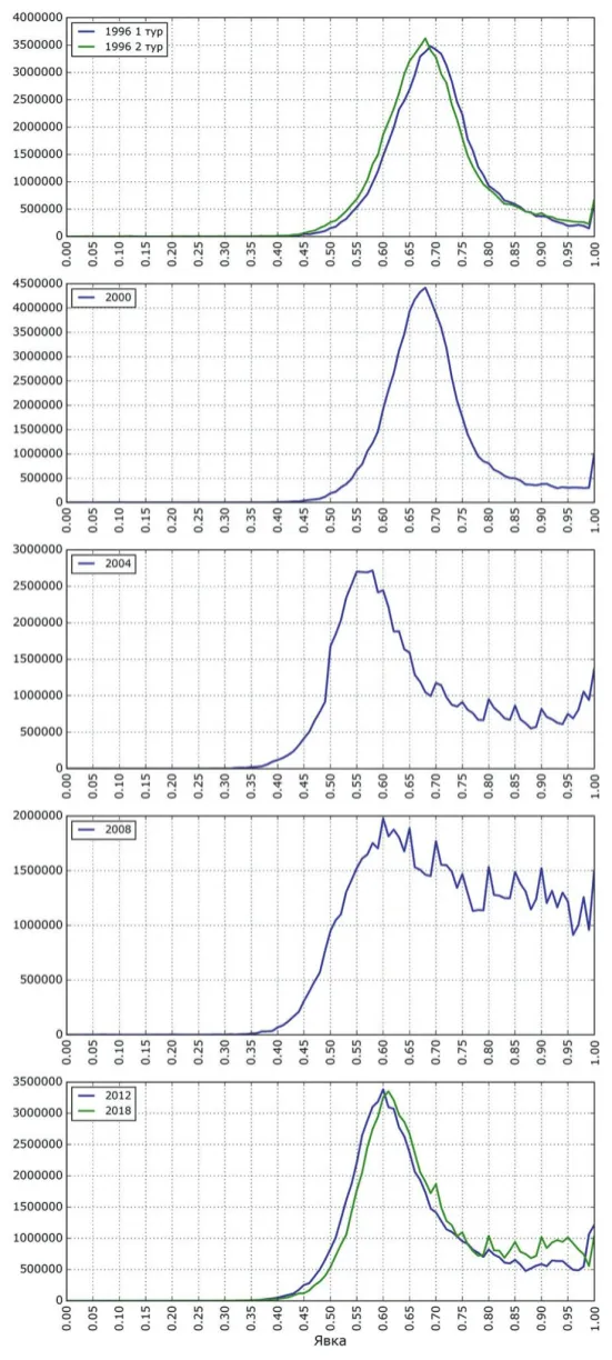Rice. 1. Distribution of votes of voters, depending on the final appearance in polling stations, presidential elections in Russia in 1996-2018. According to the abscissa axis: a turnout at the polling station (sites are grouped in the intervals of the appearance of 1% of the whole to a whole percent). According to the ordinates axis: the number of votes in the areas in the corresponding 1 % turnout interval 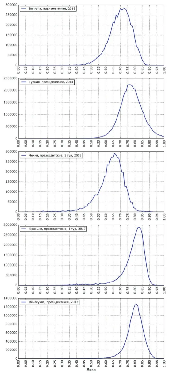Rice. 2. The same, in several foreign elections. Data from the sites of central election commissions or open data portals of relevant countries

In Fig. 1 shows (in the form of schedules) the histogram of the distribution of the number of voters voted by the final turnout in polling stations in the federal elections in Russia in 1996-2018. The curves for 2012 and 2018 are intentionally placed on one schedule to emphasize their remarkable similarity (see Figure 1 in full ).

In Fig. 2 shows similar histograms for several national elections in foreign countries ( see Fig. 2 in full ).

When comparing two drawings, a well -known characteristic feature of the Russian federal elections is clearly visible - an asymmetric distribution of turnout with a “heavy tail”: an unusually large number of polling stations (and, accordingly voters that voted on them) with appearances approaching 100%. In other countries of the “heavy tails” of distribution, reaching up to 100% turnout, except perhaps Turkey, but there this tail is significantly inferior to Russian patterns.

The simple bell -shaped form of voting distribution in the appearance observed in foreign elections is, in a sense, the most natural for the size, the value of which is affected by a large number of independent factors.

So, in the case of the election, these are, for example, demographic characteristics and political preferences of the population of a particular site, the activity of campaigning in this area, the weather on the voting day, the distance to the place of voting, etc. This is simply due to the fact that the number of combinations of factors with multidirectional deviations from the average (which contribute to the central part of the distribution) more than the number of combinations from Sonfire deviations (which form the "tails").

Accordingly, the presence of a large one -sided “tail” in the Russian elections suggests that there is a single factor (we will call it factor X), which affects the turnout towards its increase and often surpasses the total effect of other factors.

The second feature is well noticeable in the graphs for the Russian elections: unusual distribution behavior on “beautiful” percentage values ​​of the turnout. For the first time, this feature is manifested in the 2004 presidential election, and in two places at once: in the form of a characteristic “comb” with a step of 5% on the right tail of the distribution and in the form of not so noticeable, but clearly expressed “steps” in the distribution between a 49% explicit and 50%.

Recall that in 2004 the law was still in force on the verge of turnout in the presidential election (the presidential elections were considered to be at least 50%of the explicit of voters). And although the threshold was established for the whole country as a whole, and not for individual sites, there is a feeling that on a fairly large number of plots, special efforts were made to ensure that the turnout was not 49 with a small percent, but pulled over 50%.

A comb on the right tail of the distribution with peaks on the values ​​of the turnout of 75%, 80%, 85%, 90%, 95%, also leads to similar thoughts: since only integers are present in the protocols of polling stations, it is necessary to make special efforts to achieve a “beautiful” appearance - and these efforts were made on a statistically significant number of plots in the country - so much significant that the result was manifested by the result. On a common histogram.

Once in 2004, the distribution of the distribution with peaks at beautiful interest (the so -called “Churova”) does not disappear in subsequent elections (both presidential and parliamentary parliamentary ones), reaching the maximum in 2008 simultaneously with the maximum size of the right “tail” of distribution.

The article [5] showed that the distribution peaks on entire percentage are statistically significant and cannot be explained by natural factors: (by randomness, effects of integer division, etc. (see also an article [6] dedicated to the evolution of the Churov saw in the 2016 and 2018 elections). It remains to assume that the nature of these peaks is due to manual intervention in Voting protocols.

Moreover, the presence of peaks on the “beautiful” numbers makes us assume that the turnout is the subject of some administrative reporting - and this suggests that the tail of the distribution from the side of high athletes grows in parallel with the “Churov’s saw” is also a manual intervention for the sake of administrative reporting. In this case, it is natural to assume that the factor X, which generates the tail mentioned above, is precisely the administrative impact on the elections.

In order to illustrate how the factor X acts on the results of specific candidates, we will build a distribution of votes for each candidate in the same way as it was done in [2]. The relevant graphs are shown in Fig. 3 on the left. As well as on similar schedules for the elections of past years, with low devices for the distribution of votes for all candidates, they are similar to each other, and with higher (in this case, starting from the plots with a turnout of 68%) a histogram of votes for the administratively supported candidate (V. Putin) begins to deviate up from the votes for other candidates (the distinction in the form of distributions is shown by hatching).

How this happens, it can be seen from the right diagram, where points of different colors show the results of candidates in all polling stations in the coordinates of the “turnout-result”. With low athletes, the points form compact clusters corresponding to the main peak of the distribution on the left, and with higher turners they form the “tail of the comet”, which the candidate Putin goes up, and the rest of the candidates - down.

This behavior is consistent with the assumption that the “tail” is formed as a result of adding votes to the right candidate, which simultaneously leads to an increase in turnout. At the same time, the “tail” of the comet is clearly visible a characteristic “checkered” drawing due to the abnormal concentration of polling stations on the “beautiful” values ​​of the appearance and the result of the “main” candidate (another argument in favor of the “tail” is the fruit of manual intervention in the results, and not a natural education). At the level of individual regions, the voting picture looks very different (see Fig. 4.).

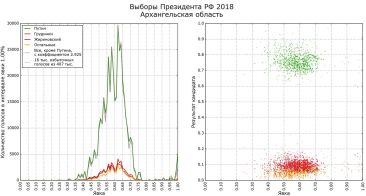
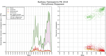
Rice. 4. Examples of vote distribution for candidates for a turnout in different regions

All regions of Russia can be divided by the nature of the distribution of votes into three groups.

• (Example: Arkhangelsk region.) In the scattering diagram, the results of all sections form a compact cluster, there is no “Kometa tail”. The distribution of votes for all candidates in the turnout has the same bell -shaped shape, the forms of distribution of votes for V. Putin and other candidates are the same.
• (Example: The Republic of Mordovia.) Some of the sites form a cluster on the same values ​​of the turnout and the result as in other regions of the country, and part of the “tail”. Within the main cluster of the distribution of votes for all candidates, the share of votes for V. Putin is greatly increased in the “tail”.
• (Example: Karachay-Cherkess Republic.) In the field of the main cluster of the sections of the whole country, only single sections are located, and most forms the “tail”. Judging by the reports of physical and video surveillanceers from the regions of this kind, the real turnout and real results correspond to precisely to the single areas with the turnout near the area of ​​the main cluster (and in many areas the appearance is much lower than the average in the country). In Fig. 5 shows the distributions of votes for the appeal candidates, built separately for these three groups of regions.

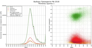
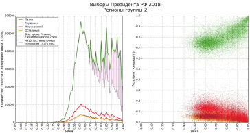
Rice. 5. Distribution of votes for candidates for a turnout in three groups of regions.
Group 1: Altai Territory, Amur Region, Arkhangelsk Region, Vladimir Region, Vologda Oblast, Trans -Baikal Territory, Ivanovo region, Irkutsk region, Kaliningrad region, Kaluga region, Kamchatka Territory, Kirov region, Kostroma region, Krasnoyarsk Territory, Kurgan Region, Leningrad Region, Magadan Region, Murmansk Region, Nenets Autonomous Okrug, Autonomous Okrug, Autonomous Okrug, Autonomous Okrug, Autonomous Okrug, Autonomous Okrug. Нижегородская область, Новгородская область, Новосибирская область, Омская область, Оренбургская область, Пермский край, Приморский край, Псковская область, Республика Карелия, Республика Коми, Республика Крым, Республика Марий Эл, Республика Саха (Якутия), Республика Хакасия, Самарская область, Сахалинская область, Свердловская область, Смоленская область, Тверская область, Томская область, Тульская область, Udmurt Republic, Khabarovsk Territory, Khanty-Mansi Autonomous Okrug-Ugra, Chelyabinsk region, Yaroslavl region, city of Moscow, the city of St. Petersburg, the city of Sevastopol, foreign plots
Group 2: Astrakhan region, Belgorod region, Bryansk region, Volgograd region, Voronezh region, Jewish autonomous region, Krasnodar Territory, Kursk region, Lipetsk region, Oryol region, Penza region, Republic of Adygea (Adygea), Altai Republic, Republic of Bashkortostan, Republic of Buryatia, Republic of Kalmykia, Republic of Mordovia, Republic of Mordovia, Republic of Mordovia, Republic of Mordovia, Republic of Mordovia, Republic of Mordovia, Republic of Mordovia, Republic Tatarstan (Tatarstan), Rostov region, Ryazan region, Saratov region, Stavropol Territory, Tambov region, Tyumen region, Ulyanovsk region, Chuvash republic - Chuvashia, Chukotka Autonomous Okrug
Group 3: Kabardino-Balkarian Republic, Karachay-Cherkessian Republic, Kemerovo Region, Republic of Dagestan, Republic of Ingushetia, Republic of North Ossetia-Alania, Republic of Tva, Chechen Republic, Yamalo-Nenets Autonomous District

In group 1 (49 regions plus foreign plots, 68.6 million registered voters) the distribution has a completely “European” look if you neglect a small tail on high attendance and small cloves on turnout 70%, 80% and 90% - even in the context of an honest calculation, some election commissions could not help the temptation to fit the turnout to beautiful values. (As it was done is a question, one of the possible options - manipulation with the list of voters).

In group 2 (28 regions, 33.9 million registered voters) the distribution of votes for candidates resembles the distribution throughout the country in the 2008 presidential election (see [2]). There is a powerful “Churov saw” - peaks on all multiple 5 percent of the turnout, starting with 70%. At the same time, the initial part of the distribution is approximately in the same place as in group 1 - that is, it is clear that, apparently, the regions of group 2 are the same regions as in group 1, but subjected to significant manipulations when counting votes.

Finally, in group 3 (9 regions, 6.45 million registered voters) , the election results are apparently falsified total (or almost total). If you look closely, in the scattering diagram you can consider the pale shadow at the place where the main cluster is located on the all -Russian diagram (a turnout is about 62%, Putin's result is about 72%). It is also noteworthy that a certain number of areas with a very low one - from 23% - a turnout. Such turnouts in the republics of the North Caucasus were really reported by both local observers and volunteers engaged in watching videos.

It is noteworthy that in the regions of the third group “Pila Churov” there is no. Apparently, here, unlike the regions of the second group, not so much “beautiful” as a high result is appreciated.

In connection with the division of regions into categories, I would like to note the number of "clean" regions for the election of recent years. The Republic of Mari El, Sakha-Yakutia, Tula Region returned to group 1. Bashkortostan and Tatarstan and even Mordovia, which was the last time there in 2000, moved to group 2 from the third.

Quantitative assessment of the level of falsification

If falsification during the calculation is made exclusively by the method of adding (stuffing or attributing) votes for the desired candidate, then the shared area (10.37 million votes) on the left schedule of Fig. 3 gives the value of the number of thrown voices. This assessment of the stuffing is obtained with a fairly general assumption about the nature of the initial distribution of votes (without a significant correlation between the shares of votes for candidates and the turnout) and the nature of falsifications (it is assumed that they are used evenly over the entire range of source areas) [2].

However, the assumption about the stuffing of 10.37 million votes leads to the conclusion that the real turnout in the elections in question was 58.1%, which clearly does not correspond to the position of the main peak (cluster) in Fig. 3, visually located approximately in a turnout 61.5%.

Meanwhile, the list of possible falsification options during the calculation is not limited to the stuffing/rovering votes. По накопленному наблюдателями опыту (в частности, по итогам сравнения выданных наблюдателям протоколов с официальными результатами, см., например, [7]) мы знаем, что помимо приписывания голосов встречается также переписывание голосов от «прочих» кандидатов «правильному» — как без изменения явки, так и с одновременным добавлением голосов и увеличением явки. Манипуляции первого рода практиковали на выборах прошлых лет, например, некоторые избирательные комиссии Санкт-Петербурга.

Отметим, что манипуляции первого рода (переписывание голосов без изменения явки) не влияют на положение избирательного участка по оси явки и потому не вносят прямого вклада в заштрихованную площадь на рис. 3. Они косвенно снижают оценку избыточного числа голосов, меняя в пользу административного кандидата соотношение голосов в основном пике распределения, которое используется в качестве базового при расчете количества аномальных голосов в «хвосте».

При манипуляциях второго рода (с одновременным увеличением явки) при перекладывании 2 * A голосов голосов в пользу административного кандидата заштрихованная площадь увеличивается на A * (1 + alpha) голосов, где alpha — коэффициент масштабирования, совмещающий распределения голосов за прочих кандидатов и административного кандидата на начальном участке. Дополнительное преимущество в 2 * A голосов над остальными у административного кандидата появляется благодаря тому, что у прочих кандидатов отбирается A голосов, а административному кандидату добавляется A голосов.

В данном случае, как указано на рис. 3, alpha = 2,686, поэтому перекладывание A голосов от других кандидатов административному кандидату вносит в заштрихованную площадь вклад 3,686 * A. Предполагая, что имели место как переброс, так и добавление голосов, и обозначая неизвестные количества переброшенных и вброшенных голосов A и B соответственно, получаем уравнение A + 3,686 * B = 10,37 млн.

Одного линейного уравнения недостаточно, чтобы найти два неизвестных. В качестве дополнительной информации можно использовать положение основного кластера избирательных участков на диаграмме рассеяния в правой панели. Центр наиболее плотного кластера (по методу [8]), охватывающего 50% зарегистрированных избирателей, соответствует явке 61,58% и результату В. Путина 73,60%.

Требование совпадения скорректированной явки и результата с этим центром дает еще два дополнительных уравнения для двух величин A и B, т. е. система становится переопределенной. Минимизируя в качестве невязки евклидово расстояние от скорректированных явки и результата до центра основного кластера, получаем такие решения наших уравнений: A = 1,05 млн голосов, B = 6,5 млн голосов. Скорректированные значения явки и результата при этих значениях A и B составляют 61,58% и 72,87%, что очень близко к центру главного кластера на диаграмме рассеяния и подтверждает самосогласованность подхода.

Resume

Какие же выводы можно сделать из анализа электоральной статистики президентских выборов 2018 года?

1. Картина голосования на выборах 2018 года получилась очень похожей на выборы 2012 года. В 49 из 85 регионов страны, охватывающих более 60% населения, статистически заметных массовых фальсификаций не было практически совсем (хотя это не значит, что не было других, менее заметных и не массовых). Кроме того, в ряде регионов 2-й группы они могли остаться за пределами региональных центров и пройти незамеченными.

2. Наблюдаемое распределение голосов соответствует добавлению за кандидата Путина дополнительных 6,5 млн голосов и перебрасыванию от других кандидатов еще 1,05 млн. В итоге дополнительное преимущество кандидата Путина над другими кандидатами за счет административного вмешательства в ход голосования составило 6,5 + 2 * 1,05 = 8,6 млн голосов.

3. Дальнейшего изучения требует фактор влияния на явку и результаты голосования нового механизма голосования по месту жительства. Кроме того, большую пользу может принести изучение оставшихся в распоряжении наблюдательского сообщества видеозаписей выборов.

Sergey Spilkin