Data analysis in Excel. Part 1

We talk about simple Excel functions with which you can start learning it

To work with data presented in tabular format, you can use programs installed on your computer - Microsoft Excel or Numbers (for Mac OS). Or use the online version of Google Sheets, which is almost similar in functionality. Toolbars differ between versions of Excel, so we'll show you how to work with this tool in Google Sheets, which looks the same on any computer.

As an example, we will use a data set with the number of sites created during the coronavirus epidemic selling medical masks in the Russian-language segment of the Internet (used in our material “Trust Deficit”).

How Excel works

The space inside the program is like a sheet of paper with squares. Each column here has its own name - according to a letter of the alphabet, and each line has its own number. Each cell has its own address, which consists of a combination of a column letter and a row number - for example, cell A1 or B2 - this is somewhat similar to the game of Battleship . The file itself is like a book with many sheets. By clicking on the plus sign in the lower left corner of the page, you can create new sheets, and for example, place each set of data on a separate sheet.

Import data

Excel works with a variety of data formats. The most common spreadsheet file extension is xlsx, which is how Excel saves data by default. To open a file in this format, you must click “File” - “Open” - and specify the path to the file.

Another common extension is csv. This is a text file in which the values ​​are separated by special characters - for example, commas (hence the name - comma-separated values) or others. It can be opened in regular Notepad. There you can view the contents of the file, but to process such data, Excel is useful. To open csv, you need to click “File” - “Import” - and specify the path to the file.

After loading, a menu will appear with the “Separator Type” section. Typically, Google Sheets will automatically detect the correct separator type, so you can leave the “Detect automatically” option checked. If the separator type is defined incorrectly, and instead of a table view you received data in an unreadable form, you can specify the separator type yourself. Select from the options provided or insert your symbol into the “Other” window. Then click “Import data” and “Open now”.

Preliminary work with data

When the data is loaded, the first thing you should check is whether it is presented in a form convenient for work. It is important, for example, to check whether columns (and sometimes rows) have names, this will simplify working with the data.

Data inside cells in Excel is presented in different formats - in our example, dates, text or numbers. All types of formats that the program works with can be seen in the “Format” menu tab. Before working with data, it is worth assessing whether its format is recognized correctly. For example, if numbers are formatted as text, they cannot be used for calculations. You can change them in the same section of the “Format” menu.

It is then important to evaluate whether the data is sufficient or worth transforming for further analysis. Let's look at our example. In the data set with the number of new sites selling medical masks, there is a column with the number of sites in the “.rf” zone, and a column with the number of sites in the “.ru” zone. We are interested in the total number of sites in both zones. You can add another column, name it “.рф and .ru” and fill it in yourself. A formula will help us add the values ​​from two columns (“.рф” and “.ru”).

Formulas

The program can use simple mathematical formulas, such as addition. You need to activate the cell that needs to be filled in (in our example D2) and enter =. It is with the equal sign that any formula in Excel begins. Then you need to indicate the address of the first cell, put +, and indicate the address of the second cell that we want to add to the first, and press the enter key (Enter or Return). The program itself will calculate the sum of two cells. You can specify as many cells in the formula as you need to add. Let’s add up the values ​​from the “mask.rf” and “mask.ru” columns. The formula will be: =B2+C2.

Autofill cells

To avoid having to perform the same operation for each date in our example, you can immediately apply the formula to the entire data range. There is a cell autofill feature for this purpose. When you select a cell in which a formula is entered, a special symbol – a square – will appear in its lower right corner. You need to hold it down, stretch it to the end of the table and then release the cursor. Then the formula will automatically be inserted into each cell of our range, and each new cell will have its own amount. The same can be done faster: double-click on the square in the lower right corner of the cell with the formula, and it will expand to the end of the table.

Functions

In the case when there is a lot of data and the formula needs to be applied to a large number of values ​​(for example, to calculate the total sum of many cells), you can use the function. Excel has many functions that allow you to perform calculations on data and process it. The entire list of functions can be viewed here .

To calculate the sum of several values, there is a special function called SUM. Let's assume that we want to calculate the sum of websites created over the entire time period available to us in the data. Type = followed by the name of the function, SUM. As soon as you start typing the name of a function, a pop-up window will appear next to it with a list of all available functions starting with those characters. If you click on the desired function from this list, it will appear in the cell, and an opening parenthesis will automatically appear after it.

Then, highlight the range of numbers that need to be added with your cursor, put a closing parenthesis and press the enter key. In our example, the function will look like this: =SUM(D2:D114). The same range of values ​​inside brackets can not be selected with a cursor, but can be specified manually in this way: address of the first cell of the range (D2), colon, address of the last cell of the range (D114).

Sorting

Sorting allows you to rearrange records in a table in a specific order - ascending or descending. In our example, the dates are not in order, and if we want to see how the situation with site registration developed from January to April, we can use sorting.

To do this, you need to select the entire table with the cursor - click on the “Data” menu - “Sort range”. Then check the “Data with header line” checkbox - this is necessary so that the headers remain in place and do not participate in sorting. Then choose by which indicator (or column heading) you want to sort the data. In our case, this is “Date”. Select the sorting type: “from A to Z” (from smallest to largest) or “from Z to A” (from largest to smallest). In our example, in order for the dates to be displayed in chronological order, we must mark “from A to Z”.

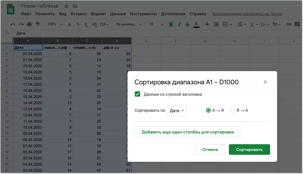
The sorting function can also be used to analyze data. For example, we are interested in what day the largest number of sites selling medical masks were registered. To do this, you need to do the same steps, but select “All sites” and “Z to A” as the sorting option. Then the maximum number of sites will be displayed at the very beginning of the table, and we will see that the peak of registration of such sites occurred on April 4.

General information about the data

The same thing can be found out in another way. Google Sheets automatically calculates the key features of your data and displays them in one place. You can select any piece of data - for example, an entire column with the number of sites - and a menu with main indicators will appear in the lower right corner of the sheet. There is a sum, an average, a maximum, a minimum and other values. This is useful to quickly get a preliminary understanding of the data.

Filtration

Filters are used to display only the data necessary for analysis and hide the unnecessary data. They also help to extract from the data only those that meet the necessary criteria, which helps with analysis. To create a filter, you need to select the table, click on the “Data” menu - “Create filter”. After this, inverted triangles will appear next to the headings of each column - this is the filtering menu.

Let's find out on which days sites selling masks were not registered. You need to click on the filtering menu in the “All sites” column. In it we will see a list of all the values ​​that are in the data set. Click on “Clear” (by default all values ​​are selected, but we need to leave only one) and select only “0”. After this, the table will change its appearance, and it will show only rows with dates when sites were not registered. For example, we will see that this did not happen during the New Year holidays.

Filtering can also be done by conditions. Let's find out on what days more than 50 sites were registered. To do this, in the filtering menu you need to select “Filter by condition”, select the “More than” condition from the list and enter the value “50” in the window. There are only three dates left when more than 50 sites were registered - these are the first three days of April.

There are other examples of conditions. For example, we want to display data for April only. In the filter menu for the “Date” column, click “Filter by condition” – “Date after” – “Exact date” – and enter “03/31/2020”. Only data for April has been displayed, and now you can begin to analyze it. For example, select this column and look at general information about the data in the lower right corner of the sheet. We will see, for example, that every day in April, on average, 34 such sites were registered.

It is important to understand that filters do not remove unnecessary data from the table, but only hide it. To keep data for April only forever, you need to save it as a new dataset. To do this, you can copy the table with the filter enabled and paste it into a new sheet.

Saving

Google Sheets, if connected to the Internet, independently saves every action and work results. If you need to save the processed data to your computer, you can do it this way: select “File” in the menu, click “Download” and select the required format from the drop-down menu - there are both xlsx and csv, as well as other formats.